In most computer vision fields, the challenge lies in algorithm development, and accessing images is straightforward. But in computational pathology, data scientists face unique hurdles. Simple tasks like storing, manipulating and loading images can be a time sink and source of frustration. Scanner vendors use proprietary file formats. Loading whole slide image (WSI) files from multiple vendors requires various code packages that are not well maintained. WSI files are storage intensive, holding gigabytes of data per file. Processing high magnification WSI files for downstream deep learning workflows requires cropping WSI files into many smaller images, turning a single WSI file into sometimes thousands of individual data products to track and maintain.
Only after overcoming these hurdles can a data scientist start to build a model for the important task at hand–whether that’s detecting a specific biomarker, identifying mitoses, classifying a tumor type, or any of the other countless uses for AI in pathology.
Transforming Computational Pathology with Concentriq® Embeddings
To help address these challenges, computational pathology AI development has recently recognized the immense potential of foundation models for accelerating downstream task-specific development. Just as language foundation models power transformative applications like ChatGPT, computer vision foundation models like DINO and ConvNext provide a state of the art approach to developing downstream AI models that perform tasks in medical image analysis. Data scientists leverage computer vision foundation models to turn cumbersome image files into standardized, lightweight feature vectors known as embeddings, which act as the building blocks for downstream AI development.
Proscia’s Concentriq® Embeddings enables data scientists to easily adopt this new mode of AI model development by empowering them to efficiently generate WSI embeddings using a collection of leading vision and vision-language foundation models directly connected to the enterprise pathology platform where their data resides. Data scientists simply assemble a WSI dataset in Concentriq and submit an API post request from a chosen foundation model, specifying the resolution, and optionally, the region of interest. The request for embeddings is sent to the chosen foundation model via the Concentriq API and tile embeddings are quickly generated and returned to the user, ready for downstream AI model development (Figure 1).

Figure 1. Workflow to generate embeddings using Concentriq Embeddings.
With Concentriq Embeddings, Proscia is putting the power of foundation models at data scientists’ fingertips to accelerate AI-enabled precision medicine breakthroughs while significantly reducing computational costs. We envision many downstream applications for AI models built with Concentriq Embeddings ranging from image classification and segmentation to risk scoring and multimodal data integration, supporting rapid prototyping and large-scale AI model development for therapeutic R&D (Figure 2).
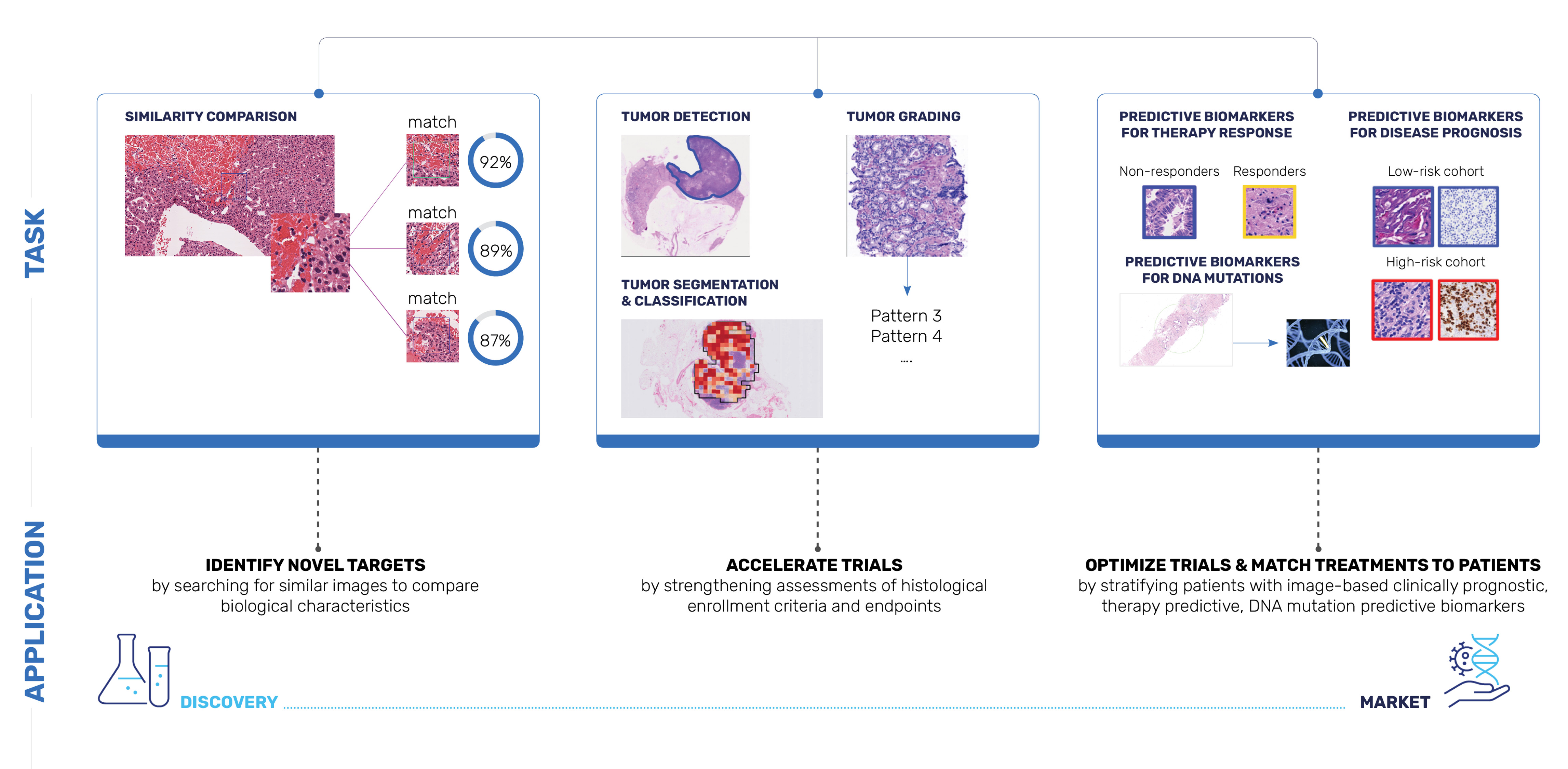
Figure 2. Potential applications for AI models built with Concentriq Embeddings.
Finally—A Straightforward Workflow for Pathology AI Development
Concentriq Embeddings, a seamless extension of Proscia’s Concentriq platform, is designed specifically for life sciences organizations to build AI models and algorithms that can be used across the R&D lifecycle to accelerate the development of precision therapies and diagnostics without the traditional barriers. Concentriq Embeddings provides foundation model embeddings from WSIs in the Concentriq platform. The service extracts rich visual features at any magnification above the base mpp, promptly providing access to the visual information in the slide, at a greatly compressed memory footprint.
Through Concentriq Embeddings, developers can access some of the most widely used foundation models, and Proscia plans to continue adding to the list of supported foundation models. Instead of wading through the ever-growing and dense literature attempting to crown a “best” foundation model for pathology, Concentriq Embeddings allows researchers to easily try out many feature extractors on a downstream task, and future-proofs for the inevitably better foundation models of tomorrow.
Currently supported foundation models include:
| DINOv2 | Model Tag: facebook/dinov2-base Patch Size: 224 Embedding Dimension: 768 🤗 HuggingFace page Paper |
| PLIP | Model Tag: vinid/plip Patch Size: 224 Embedding Dimension: 512 🤗 HuggingFace page Paper |
| ConvNext | Model Tag: facebook/convnext-base-384-22k-1k Patch Size: 384 Embedding Dimension: 1024 🤗 HuggingFace page Paper |
| CTransPath | Model Tag: 1aurent/swin_tiny_patch4_window7_224.CTransPath Patch Size: 224 Embedding Dimension: 768 🤗 HuggingFace page Paper |
Concentriq Embeddings revolutionizes the AI development process—from selecting WSIs to extracting features from them, and beyond—making downstream model and algorithm development much more straightforward.
Traditional AI Development:
Data scientists juggle countless non-standardized WSI file formats and struggle with often poorly-maintained code packages for accessing WSI files.
With Concentriq Embeddings:
Forget about OpenSlide, proprietary software development kits (SDKs) from scanner vendors, and OpenPhi. Concentriq and Concentriq Embeddings are all you need to get started with your AI development.
Traditional AI Development:
Training models with pathology images requires downloading large WSI files that require extensive storage capacity since each file often exceeds several gigabytes. This often produces more data than can be accommodated by a standard laptop hard drive. Furthermore, downloading such substantial amounts of data on a typical internet connection can take several hours or even days, significantly slowing down the research workflow and delaying critical advancements until the required expensive specialty infrastructure is implemented.
With Concentriq Embeddings:
Rather than managing slides that consume gigabytes of memory, data scientists now interact with lightweight feature representations that occupy just a few megabytes. For example, an RGB WSI crop of 512 pixels on each side contains 512x512x3= 786,432 unsigned 8-bit integers, or 786,432 bytes. In contrast, a Vision Transformer (ViT) feature vector (embedding) of this crop contains 768 floats at 4 bytes apiece, for 3,072 bytes. The feature vector is a compressed representation of the image, with a compression rate of 256! This means a 1 GB WSI becomes less than 4 MB, enabling faster, easier AI model development.
Traditional AI Development:
Preparing high magnification WSI files for downstream deep learning workflows involved cropping WSI files into many smaller images, turning a single WSI file into sometimes thousands of individual data products to track and maintain.
With Concentriq Embeddings:
Concentriq Embeddings tiles each slide and returns a single safetensor file per slide containing the embeddings, simplifying data management. Even though the slide’s visual information is contained in a single convenient file, Concentriq Embeddings provides an interface for loading feature vectors from individual crops into memory.
Tutorial: Using Concentriq Embeddings for Unsupervised Clustering
In this tutorial, we’ll walk through an example using the publicly available IMPRESS dataset, containing WSIs from breast cancer patients. We’ll use the Python client developed specifically for Concentriq Embeddings and available in the Proscia AI Toolkit to demonstrate how to request and retrieve embeddings, cluster the results, and visualize the underlying structure of the data.
Note: Here’s a video walkthrough of the tutorial if you’d like to follow along that way.
First, we’ll secure our access to Concentriq and Concentriq Embeddings.
import os

from utils.client import ClientWrapper as Client
from utils import utils

email = os.getenv("CONCENTRIQ_EMAIL")
pwd = os.getenv("CONCENTRIQ_PASSWORD")
endpoint = os.getenv("CONCENTRIQ_ENDPOINT_URL")

# To use CPU instead of GPU, set `device` parameter to `"cpu"`
ce_api_client = Client(url=endpoint, email=email, password=pwd, device=0)
Embedding the IMPRESS Dataset
The IMPRESS dataset that we’re using for this tutorial contains 126 breast H&E and 126 IHC WSIs from 62 female patients with HER2-positive breast cancer and 64 female patients diagnosed with triple-negative breast cancer. All the slides are scanned using a Hamamatsu scanner with 20x magnification. These WSIs are stored in a repository in our Concentriq instance.
To get started, we’ll submit a job for our entire dataset and request our embeddings at a scale of 1 µm/pixel (mpp).
repo_ids = [1918] # The IMPRESS Dataset
ticket_id = ce_api_client.embed_repos(ids=repo_ids, model="facebook/dinov2-base", mpp=1)
Retrieving and Understanding the Embedding Results
Now the embedding job is running and Concentriq Embeddings is running inference with our selected foundation model. With get_embeddings, we can check for completed results, and when complete they’ll get pulled down to a local cache. If the cache is already stored locally, get_embeddings will load out the results on demand from disk.
embeddings = ce_api_client.get_embeddings(ticket_id)
print(f"{ticket_id}: {len(embeddings['images'])} images")
print(f"{embeddings['images'][0]['model']} - {embeddings['images'][0]['patch_size']}")
The retrieved embedding file includes metadata about the embeddings job we submitted and each WSI processed. The embeddings themselves are loaded as a dictionary of tensors with keys in “Y_X” format indicating the grid index of the embedded patch.
Here, we print the information corresponding to each WSI. This includes the parameters supplied along with implicit attributes of the data, like the foundation model’s native patch size, as well as all of the other spatial information associated with each WSI’s tile embeddings.
for key, value in embeddings['images'][0].items():
    if key not in ['embedding']:
        print(f"{key}: {value}")
At this point, this dataset has been processed into embeddings—it’s now lightweight and ready for downstream analysis, be that classification, segmentation, regression, etc. For this example, we’ll show how to cluster similar embedding vectors and visualize the underlying tiles.
embeddings['images'][0]['embedding']['0_0'].shape
torch.Size([768])
Our embedding file also contains a lightweight thumbnail image that allows us to visualize the image tiles associated with each embedding—let’s grab that thumbnail image and tile it now as well.
thumbnail_ticket_id = ce_api_client.thumnail_repos(ids=repo_ids)
print(thumbnail_ticket_id)
thumbnails = ce_api_client.get_thumbnails(thumbnail_ticket_id, load_thumbnails=True)
# link the thumbnails to the embeddings
for emb in embeddings['images']:
    thumbnail_dict = [thumb for thumb in thumbnails['thumbnails'] if thumb['image_id'] == emb['image_id']][0]
    emb.update(thumbnail_dict)
emb = embeddings['images'][0]
tiles = utils.tile_thumbnail(emb)
emb['tiles'] = tiles
len(tiles)
4836
Visualizing and Clustering of Tile Embeddings
Using techniques like UMAP for dimensionality reduction, you can explore the underlying feature space of the embeddings and gain insights into the data, such as identifying similar tissue types across slides.
The ability to visualize embedded space in this way is invaluable for understanding the patterns and relationships captured by foundation models—without the need for heavy computing resources or extensive preprocessing.
To get started, let’s import some s/things/libraries to allow us to cluster and visualize.
import pandas as pd
import matplotlib.pyplot as plt
from matplotlib.offsetbox import OffsetImage, AnnotationBbox
import numpy as np
from sklearn.cluster import KMeans
import umap
Next, let’s do a 2D UMAP projection of the tile embeddings for a single slide to see what the data looks like.
# Do a umap 2d embedding projection of the tiles
sorted_keys, _ = utils.parse(emb['embedding'])
all_X = utils.stack_embedding(emb['embedding'], sorted_keys)
reducer = umap.UMAP(n_components=2)
embeddings_2d = reducer.fit_transform(all_X)

fig, ax = plt.subplots(1,1,figsize=(10, 10))
ax.scatter(embeddings_2d[:,0], embeddings_2d[:,1], s=0)

for (x0, y0), key in zip(embeddings_2d, sorted_keys):
    tile = OffsetImage(emb['tiles'][key], zoom=0.3)
    ab = AnnotationBbox(tile, (x0, y0), frameon=False)
    ax.add_artist(ab)

ax.axis('off')
plt.show()

Visualizing Embedded Space
Great! Now, let’s pull out a sample over the entire dataset and cluster the embeddings to explore the approximate structure of the feature space represented by the embeddings.
images = [e for e in embeddings['images']]
all_X = []
res_df = []
for image in images:
    skeys, locdict = utils.parse(image['embedding'])
    tiles = utils.tile_thumbnail(image)
    image['tiles'] = tiles
    sample_keys = np.random.choice(skeys, size=min(1000, len(skeys)), replace=False)

    image['sample_keys'] = sample_keys
    sample_X = utils.stack_embedding(image['embedding'], image['sample_keys'])
    df = pd.DataFrame({"sample_key": image['sample_keys']})
    df["image_id"] = image["image_id"]
    all_X.append(sample_X)
    res_df.append(df)

sample_df = pd.concat(res_df)
sample_df['index'] = np.arange(len(sample_df))
all_X = np.concatenate(all_X, axis=0)
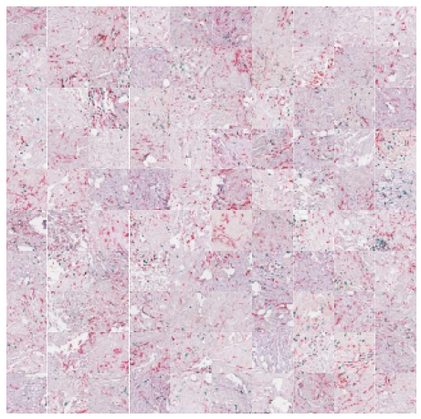
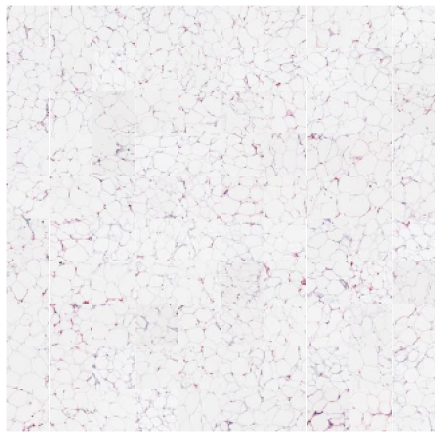
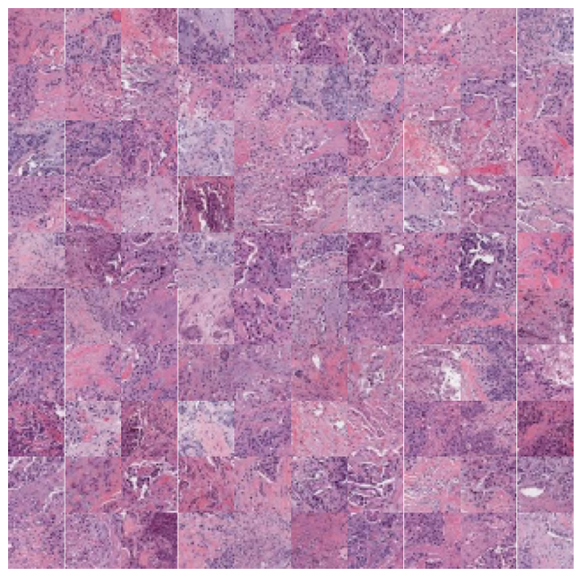
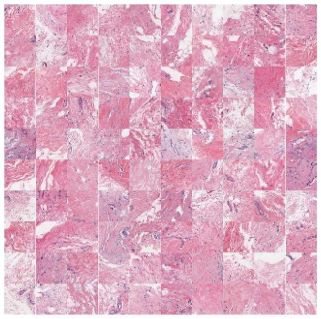
We can zoom in and visualize sample tiles from some of the clusters to confirm that the model is distinguishing relevant tissue types and structures. We’ll again use the low resolution thumbnails returned by the API to generate downsampled versions of the tiles. While these images are lower resolution (32×32 at 7 mpp) than the patches seen by the foundation model (224×224 at the requested 1 mpp), it’s easy to see that the model separates the dataset into coherent tissue and stain combinations.
n_clusters = 20
cluster_membership = KMeans(n_clusters=n_clusters, random_state=0, n_init="auto").fit_transform(all_X)
n_rows = 10
for cluster in [1,5,7,9]:
    top_n = cluster_membership[:,cluster].argsort()[:n_rows*n_rows]
    cluster_df = sample_df.iloc[top_n]
    print(cluster)
    fig, axx = plt.subplots(n_rows,n_rows,figsize=(10, 10))
    for i in range(n_rows*n_rows):
        ax = axx[i//n_rows, i%n_rows]
        ax.axis('off')
        # get the thumbnail for the key
        key = cluster_df['sample_key'].values[i]
        image_id = cluster_df['image_id'].values[i]
        emb = [e for e in embeddings['images'] if e['image_id'] == image_id][0]
        tile = emb['tiles'][key]
        ax.imshow(tile)
    plt.subplots_adjust(wspace=0, hspace=0)
    plt.show()
That’s all there is to it! That’s how easy it is to cluster and explore your data with foundation models using Concentriq Embeddings. Hello computational pathology world.
Foundation Models at Your Fingertips
Concentriq Embeddings removes the barriers between scientists and valuable insights by making grabbing features with a foundation model as easy as grabbing a cup of coffee. Data scientists can now bypass the cumbersome steps of downloading massive WSI files, wrestling with poorly maintained software, and keeping track of thousands if not millions of cropped image files that might be outdated as soon as they hit the hard drive. No heavy compute, no GPUs, no piles of harddrives. You get straight to building your models.
With Concentriq Embeddings, the barrier between your data and your models disappears, allowing you to transition seamlessly from raw slides to features ready for downstream AI development. Get ready to unlock the next generation of computational pathology—quickly, easily, and cost-effectively.
To learn more, check out additional tutorials available in the Proscia AI Toolkit, access the code for this tutorial, or visit the Concentriq Embeddings page.
Corey Chivers, Ph.D. is a Senior AI Scientist at Proscia
Vaughn Spurrier, Ph.D., is an AI Research Team Lead at Proscia
Julianna Ianni, Ph.D., is the Vice President, AI Research & Development at Proscia
