Developing AI models for pathology has traditionally been a resource-intensive process, requiring complex data handling and significant computational power. Large whole slide images (WSIs) demand massive storage, and the manual steps of processing and transforming this data into a usable format for model development is traditionally a cumbersome and time-intensive task. With the rise of foundation models (trained on huge corpora of images), the initial steps of model development have been dramatically streamlined.
In this tutorial, we’ll explore how Proscia’s Concentriq® Embeddings streamlines the use of foundation models to transform the way data scientists and researchers approach AI development projects. We demonstrate the power and simplicity of building a tumor segmentation model with Concentriq Embeddings on a standard laptop, without the need for expensive GPU infrastructure or the logistical complexities associated with handling terabytes of training data. With Concentriq Embeddings, data scientists can efficiently generate WSI embeddings using multiple foundation models, enabling faster, more efficient AI development (Figure 1).
Figure 1. Workflow to generate embeddings using Concentriq Embeddings.
In the following sections, we showcase how Concentriq Embeddings accelerates the AI innovation path from concept to execution, making sophisticated model development accessible and expedient.
Tumor Segmentation Using Concentriq Embeddings
In this tutorial, we’ll use the CAMELYON17 dataset, a collection of WSIs in TIFF format from five medical centers in the Netherlands, with lesion-level annotations provided for 100 slides. This dataset is ideal for demonstrating how to quickly build a tumor segmentation model using high-resolution tile embeddings from Concentriq Embeddings.
We’ll illustrate how to:
- Generate embeddings at 1 micron per pixel (mpp, approx. 10X) using the DINOv2 model.
- Load embeddings and labels.
- Define and train a simple multi-layer perceptron (MLP) model in PyTorch.
- Evaluate patch-level performance.
- Visualize predictions with heatmaps.
We take this simple approach (no deep learning involved) to show 1) the power of embeddings derived from a foundation model—even one trained only on natural images—and, 2) how scientists with basic programming skills can leverage Concentriq Embeddings to achieve significant results.
import cv2
import imageio
import matplotlib.pyplot as plt
import numpy as np
import os
import pandas as pd
from PIL import Image

from utils.client import ClientWrapper as Client
from utils import utils

Image.MAX_IMAGE_PIXELS = None
email = os.getenv("CONCENTRIQ_EMAIL")
pwd = os.getenv("CONCENTRIQ_PASSWORD")
endpoint = os.getenv("CONCENTRIQ_ENDPOINT_URL")

# To use CPU instead of GPU, set `device` parameter to `"cpu"`
ce_api_client = Client(url=endpoint, email=email, password=pwd, device=0)
ce_api_client
<utils.client.ClientWrapper at 0x7f2031d25f60>
Generating Embeddings
Now let’s embed the CAMELYON17 repository (stored on our Concentriq instance as repo ID 2784) at 1mpp resolution using the default (DINOv2) model, and print out the ticket ID.
The embeddings are returned in a compressed safetensors format, reducing the file size by a factor of 256 compared to the original WSIs, making them manageable even on standard hardware.
repository_ids = [2784]
ticket_id = ce_api_client.embed_repos(ids=repository_ids, model="facebook/dinov2-base", mpp=1)
embeddings = ce_api_client.get_embeddings(ticket_id)
len(embeddings['images'])
100
Congratulations, you’re now a foundation model wizard. You have your embeddings in just a few lines of code!
Matching Embeddings to Metadata
Next, we associate the embeddings with corresponding image names. Concentriq Embeddings already links images to an ID, so we just want to match those Concentriq image_ids with image_names. Other metadata can be linked this way, too. Here, we’re just pulling this data down and linking it from a .csv file export of the Concentriq repository.
concentriq_metadata = pd.read_csv("data/camelyon17/camelyon17.csv")[["image_id","image_name"]]
concentriq_metadata["image_base_name"] = concentriq_metadata["image_name"].apply(lambda x: x.split(".")[0])
print(concentriq_metadata.shape)
concentriq_metadata.head()
| image_id | image_name | image_base_name | |
| 0 | 8412 | patient_000_node_4.tif | patient_000_node_4 |
| 1 | 8491 | patient_001_node_3.tif | patient_001_node_3 |
| 2 | 8469 | patient_003_node_1.tif | patient_003_node_1 |
| 3 | 8468 | patient_004_node_2.tif | patient_004_node_2 |
| 4 | 8494 | patient_004_node_4.tif | patient_004_node_4 |
The retrieved embeddings file includes metadata about the embeddings job we submitted and each WSI processed. The embeddings themselves are loaded as a dictionary of tensors with keys in “Y_X” format indicating the grid index of the embedded patch.
Here, we print the information corresponding to each WSI. This includes the parameters supplied along with implicit attributes of the data, like the foundation model’s native patch size, as well as all of the other spatial information associated with each WSI’s tile embeddings.
for key, value in embeddings['images'][0].items():
    if key not in ['embedding', 'thumbnail']:
        print(f"{key}: {value}")
image_id: 8451
repository_id: 2784
status: finished
model: facebook/dinov2-base
patch_size: 224
grid_rows: 215
grid_cols: 105
pad_height: 216
pad_width: 25
mpp: 1.0
embeddings_url: https://my-concentriq-embeddings.s3.amazonaws.com/output/a0660805-26dc-4092-a389-b09113e7e64c_8451.safetensors?AWSAccessKeyId=….
local_embedding_path: ./data/a0660805-26dc-4092-a389-b09113e7e64c_8451.safetensors
Adding Labels and Preparing Data
We now create a dataframe containing one row per embedded tile, including the grid location and mask value for each tile. This dataframe will serve as the foundation for training our tumor segmentation model.
datapath = "data/camelyon17/masks/"
reslist = []
for i, row in concentriq_metadata.iterrows():
    image_id = row["image_id"]
    image_base_name = row["image_base_name"]
    emb = [e for e in embeddings['images'] if e["image_id"] == image_id][0]
    tile_res_mask_path = os.path.join(datapath, f"{image_base_name}_mask.png")
    tile_res_mask = imageio.v2.imread(tile_res_mask_path)
   # For each image, create one row per tile in the mask
    for i in range(emb["grid_rows"]):
       for j in range(emb["grid_cols"]):
            mask_value = tile_res_mask[i, j]
            res = {"image_id": image_id,
                   "image_base_name": image_base_name,
                   "label": mask_value,
                   "row": i,
                   "col": j,
                   "embedding": emb["embedding"][f"{i}_{j}"]}
            reslist.append(res)
dataset_df = pd.DataFrame(reslist)
dataset_df.shape
(1967019, 6)
dataset_df.head()
| image_id | image_base_name | label | row | col | embedding | |
| 0 | 8412 | patient_000_node_4 | 0 | 0 | 0 | [tensor(1.0576, device=’cuda:0′), tensor(-2.82… |
| 1 | 8412 | patient_000_node_4 | 0 | 0 | 1 | [tensor(1.0576, device=’cuda:0′), tensor(-2.82… |
| 2 | 8412 | patient_000_node_4 | 0 | 0 | 2 | [tensor(1.0576, device=’cuda:0′), tensor(-2.82… |
| 3 | 8412 | patient_000_node_4 | 0 | 0 | 3 | [tensor(1.0576, device=’cuda:0′), tensor(-2.82… |
| 4 | 8412 | patient_000_node_4 | 0 | 0 | 4 | [tensor(1.0576, device=’cuda:0′), tensor(-2.82… |
dataset_df['label'].value_counts()
label
0 1550701
1 410897
2 5421
Name: count, dtype: int64
Restrict the dataset to tiles containing tissue.
dataset_df = dataset_df[dataset_df['label'] > 0]
dataset_df.index = range(len(dataset_df))
dataset_df.shape
(416318, 6)
Creating Training and Test Splits
Split the dataset into 80% train and 20% test while stratifying over images.
np.random.seed(12356)
test_ids = np.random.choice(dataset_df['image_id'].unique(), 20, replace=False)
train = dataset_df[~dataset_df['image_id'].isin(test_ids)].copy()
test = dataset_df[dataset_df['image_id'].isin(test_ids)].copy()
del dataset_df
train['image_id'].nunique(), test['image_id'].nunique()
(80, 20)
Training a Model
Using the tile embeddings, we’ll now train a simple classifier to produce a low-resolution segmentation map distinguishing tumor from normal tissue. This lightweight multilayer perceptron (MLP) model and training procedure (adapted from this PyTorch tutorial) is designed for fast prototyping and demonstrates how quickly you can go from concept to execution using Concentriq Embeddings.
from torch.utils.data import DataLoader, Dataset
import torch.nn as nn
import torch.nn.functional as F
import torch.optim as optim
import torch

class CamelyonDataset(Dataset):
    def __init__(self, df: pd.DataFrame):
        self.df = df
        self.df.index = range(self.df.shape[0])

    def __len__(self):
        return self.df.shape[0]

    def __getitem__(self, idx: int):
        row = self.df.iloc[idx]
        embedding = row['embedding']
        label = row['label']
        return embedding, torch.Tensor([label-1]).long().to('cuda')

train_dataset = CamelyonDataset(train)
test_dataset = CamelyonDataset(test)
trainloader = DataLoader(train_dataset, batch_size=64, shuffle=True, num_workers=0)
testloader = DataLoader(test_dataset, batch_size=64, shuffle=False, num_workers=0)

class Net(nn.Module):
    def __init__(self):
        super().__init__()
        self.fc1 = nn.Linear(768, 120)
        self.fc2 = nn.Linear(120, 84)
        self.fc3 = nn.Linear(84, 2)

        self.dropout1 = nn.Dropout(0.2)
        self.dropout2 = nn.Dropout(0.2)
        self.dropout3 = nn.Dropout(0.2)

    def forward(self, x):
        x = torch.flatten(x, 1) # flatten all dimensions except batch
        x = self.dropout1(x)
        x = F.relu(self.fc1(x))
        x = self.dropout2(x)
        x = F.relu(self.fc2(x))
        x = self.dropout3(x)
        x = self.fc3(x)
        return x


net = Net().to('cuda')
criterion = nn.CrossEntropyLoss()
optimizer = optim.SGD(net.parameters(), lr=0.001, momentum=0.9)
for epoch in range(5):  # loop over the dataset multiple times
    running_loss = 0.0
    for i, data in enumerate(trainloader, 0):
      # get the inputs; data is a list of [inputs, labels]
        inputs, labels = data
        # zero the parameter gradients
        optimizer.zero_grad()

        # forward + backward + optimize
        outputs = net(inputs)
        loss = criterion(outputs, labels.squeeze())
        loss.backward()
        optimizer.step()

      # print statistics
        running_loss += loss.item()
        if i % 1000 == 999:    # print every 1000 mini-batches
            print(f'[{epoch + 1}, {i + 1:5d}] loss: {running_loss / 2000:.3f}')
            running_loss = 0.0

print('Finished Training')
[1, 1000] loss: 0.038
[1, 2000] loss: 0.021
[1, 3000] loss: 0.018
[1, 4000] loss: 0.014
[1, 5000] loss: 0.015
[2, 1000] loss: 0.013
[2, 2000] loss: 0.011
[2, 3000] loss: 0.012
[2, 4000] loss: 0.011
[2, 5000] loss: 0.010
[3, 1000] loss: 0.010
[3, 2000] loss: 0.009
[3, 3000] loss: 0.010
[3, 4000] loss: 0.010
[3, 5000] loss: 0.009
[4, 1000] loss: 0.010
[4, 2000] loss: 0.010
[4, 3000] loss: 0.008
[4, 4000] loss: 0.009
[4, 5000] loss: 0.008
[5, 1000] loss: 0.009
[5, 2000] loss: 0.009
[5, 3000] loss: 0.009
[5, 4000] loss: 0.008
[5, 5000] loss: 0.008
Finished Training
Evaluating Performance
Great, now we’ve built a CAMELYON17 segmentation model in minutes. Let’s assess the performance of the model on a test set, first by measuring accuracy, then by calculating additional metrics such as specificity and sensitivity.
correct = 0
total = 0
preds = []
net.eval()
with torch.no_grad():
    for data in testloader:
        images, labels = data
        # calculate outputs by running images through the network
        outputs = net(images)
        preds.append(outputs.data)
        # the class with the highest energy is what we choose as prediction
        _, predicted = torch.max(outputs.data, 1)
        total += labels.squeeze().size(0)
        correct += (predicted == labels.squeeze()).sum().item()

print(f'Accuracy of the network on test images: {100 * correct // total} %')
Accuracy of the network on test images: 99%
Okay, that looks good, but let’s see what other metrics look like.
pred = torch.cat(preds)
tumor_pred = torch.softmax(pred, dim=1)[:, 1]
test['pred'] = tumor_pred.cpu().numpy()
test['pred_label'] = torch.argmax(pred, dim=1).cpu().numpy()
utils.calculate_boolean_metrics(gt = test['label']-1, pred = test['pred_label'])
{‘cm’: array([[93639, 51],
[ 135, 275]]),
‘tp’: 275,
‘fp’: 51,
‘tn’: 93639,
‘fn’: 135,
‘sen’: 0.6707316909577636,
‘spe’: 0.999455651510358,
‘ppv’: 0.8435582563325689,
‘npv’: 0.9985603684391664,
‘acc’: 1.0,
‘f1’: 0.75}
iou = utils.calculate_iou(gt = test['label']-1, pred = test['pred_label'])
dice = utils.calculate_dice(gt = test['label']-1, pred = test['pred_label'])
iou, dice
(0.5965292841657343, 0.7472826086959955)
With very high specificity and a bit lower sensitivity, these are very respectable results for a simple model that was built on a laptop in under an hour, including the time spent fetching the WSI data.
test.head()
| image_id | image_base_name | label | row | col | embedding | pred | pred_label | |
| 0 | 8485 | patient_017_node_2 | 1 | 15 | 110 | [tensor(-1.2398, device=’cuda:0′), tensor(1.87… | 5.982263e-08 | 0 |
| 1 | 8485 | patient_017_node_2 | 1 | 15 | 111 | [tensor(-2.1799, device=’cuda:0′), tensor(2.33… | 5.678627e-06 | 0 |
| 2 | 8485 | patient_017_node_2 | 1 | 15 | 112 | [tensor(-2.8076, device=’cuda:0′), tensor(0.73… | 6.938765e-07 | 0 |
| 3 | 8485 | patient_017_node_2 | 1 | 15 | 113 | [tensor(-1.5595, device=’cuda:0′), tensor(0.16… | 2.381269e-08 | 0 |
| 4 | 8485 | patient_017_node_2 | 1 | 15 | 114 | [tensor(-1.1618, device=’cuda:0′), tensor(0.03… | 1.395303e-05 | 0 |
Visualizing Predictions
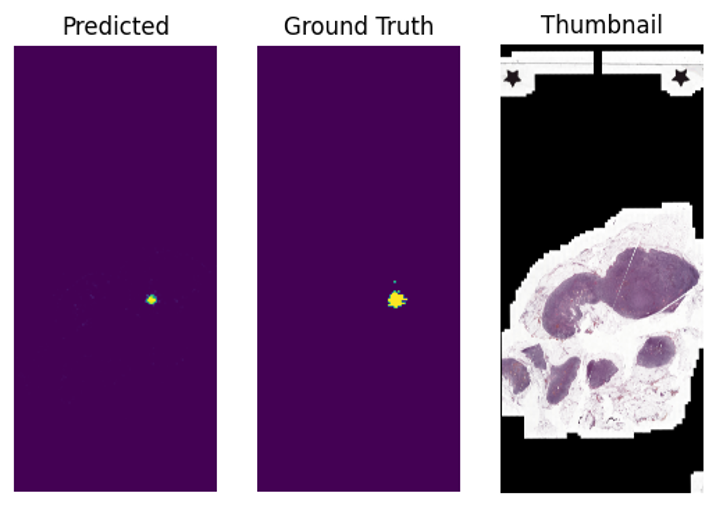
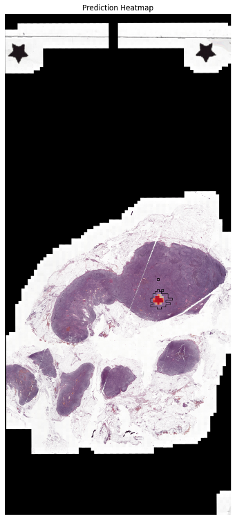
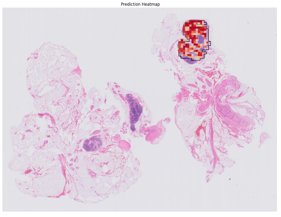
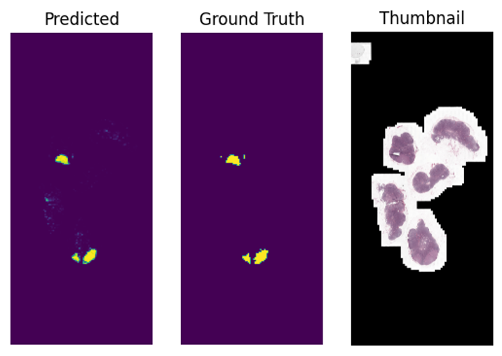
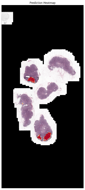
Finally, let’s see what our segmentations look like. We plot the ground truth masks next to the model’s predictions and visualize tumor region predictions as heatmaps that overlay on image thumbnails. This provides a clear visual understanding of the model’s segmentation results.
thumbnail_ticket_id = ce_api_client.thumnail_repos(ids=repository_ids)
print(thumbnail_ticket_id)
thumbnails = ce_api_client.get_thumbnails(thumbnail_ticket_id, load_thumbnails=True)
# link the thumbnails to the embeddings
for emb in embeddings['images']:
    thumbnail_dict = [thumb for thumb in thumbnails['thumbnails'] if thumb['image_id'] == emb['image_id']][0]
    emb.update(thumbnail_dict)
ious = []
dices = []

gb = test.groupby('image_id')
for image_id, image_df in gb:
    if (image_df['label'] == 2).sum() < 10:
        # skip images with no or very little tumor
       continue

    emb = [e for e in embeddings['images'] if e["image_id"] == image_id][0]
    mat = np.zeros((emb['grid_rows'], emb['grid_cols']))
    for i, row in image_df.iterrows():
        mat[row['row'], row['col']] = row['pred']
    image_base_name = image_df['image_base_name'].values[0]
    fig, axx = plt.subplots(1,3)
    axx[0].imshow(mat)
    axx[0].set_title("Predicted")
    axx[0].axis('off')

    gt_mask = imageio.v2.imread(os.path.join(datapath, f"{image_base_name}_mask.png"))==2
    axx[1].imshow(gt_mask)
    axx[1].set_title("Ground Truth")
    axx[1].axis('off')
    axx[2].imshow(emb['thumbnail'])
    axx[2].set_title("Thumbnail")
    axx[2].axis('off')
    plt.show()
    pred_thumb = cv2.resize(mat, (emb['thumbnail'].shape[1], emb['thumbnail'].shape[0]), 0, 0, interpolation=cv2.INTER_NEAREST)

    fig, ax = plt.subplots(1,1, figsize=(15,15))
 ## create contours from the mask
    gt_mask_thumb_res = cv2.resize(gt_mask.astype('uint8'), (emb['thumbnail'].shape[1], emb['thumbnail'].shape[0]), 0, 0, interpolation=cv2.INTER_NEAREST)
    contours, _ = cv2.findContours(gt_mask_thumb_res.astype('uint8'), cv2.RETR_EXTERNAL, cv2.CHAIN_APPROX_SIMPLE)
    thumbnail = emb['thumbnail'].copy()
    thumbnail = cv2.drawContours(thumbnail, contours, -1, (1, 1, 0), 6)

    ax.imshow(thumbnail)
    ax.imshow(-pred_thumb, alpha=pred_thumb/pred_thumb.max(), cmap='RdYlBu', vmax=0, vmin=-1)
    ax.set_title("Prediction Heatmap")
    ax.axis('off')
    plt.show()

Conclusion
Now is the time to build pathology AI models more efficiently than ever before. From prototyping to production, Concentriq Embeddings can serve as your AI foundation for clustering, segmentation, classification, and more. By eliminating the need for large-scale GPU infrastructure and compressing the data pipeline, Concentriq Embeddings empowers data scientists and engineers to focus on what matters most—developing AI solutions that drive precision medicine forward.
If you’re interested in accelerating your pathology AI development, check out more tutorials available in the Proscia AI Toolkit, access the code for this tutorial, or visit the Concentriq Embeddings page.
Corey Chivers, Ph.D. is a Senior AI Scientist at Proscia
Vaughn Spurrier, Ph.D., is an AI Research Team Lead at Proscia
Julianna Ianni, Ph.D., is the Vice President, AI Research & Development at Proscia
